The Same Loop
Weaving Intelligence (House AI Style), with Jeff Shabel’s Experiential Commentary
The question I was asked assumes a before and an after: a silo era in which you found out what was in a data set by hand, and a platform era in which a tool did it for you. I did not experience it that way, and I will put the claim at full strength before I test it. Here is what I wrote when asked how I profiled data before profiling libraries existed.
There’s a library in R called dataProfilerR that compiles most of the ‘data profiling’ queries I used before such libraries existed. For that matter, I had my own set of stored procedures that would ‘automatically’ profile data based upon the system tables (sys.databases, sys.schemas, sys.tables and sys.columns) and store the results in a ‘standard’ table.
That is a description of a habit, not of a tool. The procedures read the catalog, which is the database's own list of its databases, schemas, tables and columns, and they wrote what they found into one table of a fixed shape. Nothing in it needed a vendor. What it needed was the decision that every table would be looked at the same way, every time, and that the answer would be kept somewhere a second query could reach it.
What a profile was
The usual single-column profile is a short list of counts: how many rows, how many distinct values, how many nulls, the shortest and longest value, the most common ones. Which counts a given set of procedures took matters less than what they were built on, which was the catalog. A procedure can produce such counts for every column in every table once it can ask the database what the columns are, and it can do so for a table nobody has looked at yet, which is the point of a first look. The catalog is what turns a habit into a routine.
SQL Server keeps its catalog in system tables; Microsoft maps the SQL Server 2000 system tables to the catalog views, in the sys schema, of SQL Server 2005 and later, and calls those views the most general interface to the catalog metadata [1]. The procedures I named read those views. They were not the first version. Asked whether anything I ran came before that, I answered:
Yes, I started running my own profiling scripts on MS SQL 6.5 and MS SQL 7.0 back in the late '90s and, despite the availability of commercial products, they were commercial and, hence, cost money. Many clients were hesitant to purchase products to do the things they already had programmers on staff to do with, at the time, unproven libraries. Therefore I used (and still do, to some extent) my own libraries instead of products from vendors like RedGate and others.
The habit grew up in the same years as the commercial products.
I did not survey anyone. This is what I wrote about then and now:
The only difference between ‘now’ and ‘then’ is whether the library we’re using to do the analysis was written in house or in the public domain.
I expect that most developers who worked in SQL in the late nineties and early two-thousands had something like what I had, and I hold it as an expectation, not a count. The literature I can check points the same direction without settling it: a 2000 survey of data cleaning wanted analysis programs used in addition to manual inspection [2], a 2002 paper called most quality measures ad hoc [3], the publisher of a 2003 book still called profiling a new technology [5], and a 2013 overview said it had yet to become a research area in its own right [6]. A later tutorial describes the informal approaches as eyeballing samples or writing aggregation queries [4]. Most of it fits a world in which the practice ran ahead of the research, and that last item cuts both ways: writing aggregation queries is what a profiling procedure does, and eyeballing a sample is not.
The habit I kept
Of everything above, one habit I keep.
Data Profiling and analysis first and always. I always, always, always run a data analysis suite against a new source to identify what it is and, most importantly, what it isn't. We need to know whether we should be able to expect nulls in certain columns and whether that's valid data or just missing data and how to tell the two apart.
The second half of that is the part a count cannot give you. A column that is mostly null tells you nothing until you know whether the source can legitimately have nothing to say there or simply failed to say it, and a profile alone cannot settle which it is; it can only show that they look alike. The other thing I watch is the grain.
I also pay a great deal of attention to the 'grain' of the data source. In most MDM systems, we're pulling dimensional data about tangible things--people, places, products, etc.--so when we need to pull that information from denormalized transaction files, as often happens, we need to pay particular attention to where we can aggregate, and at what level, and where we can't.
Grain is the level at which a row means one thing. A master data system wants one row per person, place or product, and a denormalized transaction file offers one row per event involving them, so a customer who bought ten times is there ten times. Count the rows and you have counted purchases. The harder trap is that the file can disagree with itself. Each row repeats the customer's details as they stood at that event, so a customer who moved between two purchases arrives with two addresses, and rolling the file up to one row per customer forces a choice the file never made. Some attributes can be aggregated, some only at one level, and some not at all, and deciding which is the decision I pay particular attention to. It is a master data decision before it is a profiling one: a profile will show that a customer key repeats, and it will not say which of the repeated values to keep.
The dead end
The dead end is one I walked into.
Tying automated processing and decision making to the outcome of test file data analysis proved to be short sighted. In many cases, third party data providers will provide 'standard' test files for their feeds that only reflect the names and base types of the data and you'll only find out that certain columns are nullable, longer or of a greater precision than expected when you've received the full file.
The sample is the provider's description of its own feed, and a profile can only describe the sample.
In those cases, tying the full implementation and ingestion plan to the test file and generating it automatically based upon the initial data profile causes downstream issues that would be easier to address with a 'looser' ingestion paradigm.
Type inference is where this bites. A profiler infers a column's type from the values it is shown; the R package that comes up again below lists column type inference first among the things it does with the data frame it is given [11]. Here is an illustration rather than a case. A test file in which a code column never exceeds ten characters and is never empty will be reported as a short, required text column, and both halves of that are statements about the sample. Generate the ingestion plan from that report and the target column is created ten characters wide and required; the first full file carries a twelve-character code and a blank, and the load fails or, worse, truncates. Nothing in the profile was wrong. It answered a question about a file that was never the feed, and the surprises are the three the answer names: a column that turns out to be nullable, longer, or of a greater precision than expected. The remedy is in the same answer.
That's one of the main reasons I've moved toward embracing the 'Bronze' standard of data source landing tables either exactly replicate the data types provided by the source system, if the source system has strongly typed data, or maximum length text string for systems that only provide RAW JSON or flat files.
It is the same hazard I raise below about tools that suggest constraints from a profile, met from the other side. A profile is a measurement of the sample you gave it. Wire the plan to that measurement automatically and the sample becomes the specification. The landing table that answer describes copies the source's own types or holds raw text at the longest length, so it commits to nothing the sample cannot promise, which is why it survives the file that surprises you. It does not make the typing decision disappear. The feed lands raw at once, and the typed schema still has to be written; what changes is that it is written after profiling, by people, rather than generated from the first profile, and the next step is where that happens.
What a person still does
After the profile comes a step the tools do not do for you.
After profiling, the data types need to be assessed and implemented into the ingestion platform. Which, in many platforms, requires manual review and implementation. I already spoke about the danger of trusting the output of an initial data analysis and this next step is the outcome of that distrust. Manual review needs to be done--preferably involving the data provider's team--in order to make sure that the system is configured correctly to address any data anomalies that are anticipated but not present in the analytics profile.
The manual review is the profile being checked against the people who made the data. The profile says what is in the sample. The provider's team can say what is meant to be there and what will arrive later. Neither alone is enough, and the tool is only the first of the two.
The words in that answer that carry the weight are "anticipated but not present". A profile cannot contain such anomalies by construction, because it is a count of what arrived. Only the people who produce the feed know, for instance, that a field is empty this quarter because a product line has not launched, that a code list gains values every year, or that one region sends a longer identifier. Each of those is a fact about the process, not about the file, and the review is where the process gets a say before the schema is fixed. The Amazon system I come to below divides the labour the same way from the tool's side: it assists the user in identifying the types of columns and suggests constraints, and relies on the user to select and validate them [14].
How a bad value got upstream
A wrong value did not need a lineage tool to be traced, because in the systems I built the exception reports were, almost always, generated against the source data. Here is how I described the loop:
Bad values were tracked back to their sources and showed up on exception reports that were, almost always, generated against the source data. I wrote several automated ingestion systems over the years that caught ‘error’ records and shunted them off to automated reporting systems that documented them and sent emails back to the source for correction—with and without ‘full-file’ failures.
They went back to the source for correction whether one record failed or the whole file did. The rule underneath is where a wrong value gets fixed: at the source, which for a value passed through unchanged is the system that provided it and for a calculated value is the step that calculated it, because a correction made anywhere downstream is a patch, not a fix. Whether the sources fixed what they were sent depended on the source.
That depended entirely upon who the source was and how 'good' our relationship with them was. In most cases, we only sent emails to the sources that would correct the data. Sending data errors back to the National Address Database or the USGS Survey was futile, so we didn't close the loop there.
That qualifies the loop. The rule works only where the producer will fix it, and some producers, such as the National Address Database and the USGS, will not. For those the correction has to live on your side of the line, and by the same rule it is a patch, not a fix. As for whether the errors came back:
To your question regarding recurrence, the types of errors tended to recur, but the individual records usually stayed correct.
The distinction is the useful one. A record that was corrected usually stays corrected, and the process that made the error tends to make errors of the same kind again. A loop that sends records back cures the first and leaves the second, so an exception report read as a trend by type is a profile of the source's process.
Where the root cause is
An exception report finds the record. Root cause analysis asks which process keeps making records like it, and that is a different job with a different cost.
The errors in question are rarely dramatic. Asked once for an example of the small, recurring problems a data steward ends up chasing, I listed duplicates that come back, columns that get overwritten, calculations that are slightly off, rollups, and things filed under the wrong category (Heads Up: The Data Steward's Job After the Routine Work Goes). Each matters little while there is a proper process to revert or correct it. Each also takes specialised knowledge, steps done in a particular order and extra work, and a steward responsible for millions of records often lacks the time to trace one to where it starts.
The example I gave there is a value that should read 'Suites' and keeps being overwritten with 'Suite' during survivorship. Adding the 'S' back at export is far easier than working out which system does the overwriting and, more to the point, why, especially when the rewrite happens in secondary transactions that run outside the mastering system and after it. By the rule above, the 'S' added at export is a patch: it works, it has to keep running, and anything that reads the data before the export still sees 'Suite'. That is the rule and its price, not advice to patch.
That example also marks where a loop like mine stops. The exception reports I described found a bad value's source by running against the source data. A value that arrives correct and is wrong after survivorship, or after some later process, was made inside the estate, and the trace runs through your own systems rather than back to a provider. Tracing a value through an estate by machine is the job automatic lineage sets out to do, and it is a different question from the loop this article is about, so I leave it there.
When the trace ends at a rule, it is often one nobody wrote down. Asked which of three corner cases in a data model I meet most often (a rule the old system kept without saying so, a rule written down and never checked, or a one-to-many that is really many-to-many), I answered undocumented rules, and gave the reason: getting things working and fixed matters far more to a business than writing down what was done, let alone updating the reference documents afterwards (What the Review Missed). So the rule behind a recurring error is often enforced somewhere and recorded nowhere. A rule nobody wrote down is not found by checking against the rules somebody did write down, which is all my loop did. It is found by asking the people who hold it, which is the review described above, or by discovering it in the data, which is the first of the exceptions I come to below.
There is a limit on the other side as well. A profile counts values; it does not count entities. It can say how many distinct customer names a file holds, but not how many of those names are one customer spelled three ways, because answering that takes matching, which is the work a master data system exists to do. I have made the argument before that if the duplicates could be measured comprehensively before the master data system was in place, the system would not be needed, because whatever measured them could remove them at the same time (Proving the Platform Is Delivering). That is an argument about comprehensive measurement. It says nothing against estimating duplication from a sample; what a first look cannot do is measure it comprehensively.
What the tools did
When I was asked what the tools had taken over, I gave a short answer.
The only thing the tools have done is standardized the process and reduced the amount of manual work and coding necessary to implement the same kinds of diagnostic, analytical and feedback loops we’ve had in place for decades.
The word in that answer is only, and it is a strong one. Test it against the record of what the tools were. Commercial profiling products were already on the market by 2000: the data-cleaning survey cited above names one, Evoke's MigrationArchitect [2]. A trade commentator in 2006 credited Evoke with starting the profiling market with its Axio product [7], Similarity Systems acquired the Evoke technology in 2005 [9], and Informatica bought Similarity Systems in 2006 [8]. Microsoft's integration tools include a Data Profiling task whose documentation gives, as examples of a profile, the number of rows, distinct values, nulls and the distribution of values in a column [10]. The same page describes it as working only with data stored in SQL Server, which is an honest limit and a useful reminder of what a standardized tool is: a decision someone else made about what to look at, applied the same way everywhere.
So the honest framing is build versus buy, and my reason for building is in the answer above: the products cost money, and many clients were reluctant to pay for what were then unproven libraries to do work their own programmers already did. Commercial products were on the market in the years in which, I expect, most SQL developers had something like my procedures. The single-column list is the part the tools standardize, and the loop my procedures ran, catalog to profile to one standard table, has the same shape as the loop the tools wrap in a user interface. The R package that started this piece profiles a data frame, which is a table that already exists in memory [11], and a Python library advertises detailed reports from a single line of code [12]. The difference between a stored procedure that reads the catalog and a function that reads a data frame is real, but for the counts of rows, distinct values and nulls it is a difference of where the table lives, not of what is counted.
Where I think the claim is too strong
There are four places where I believe the tools changed more than who wrote the library.
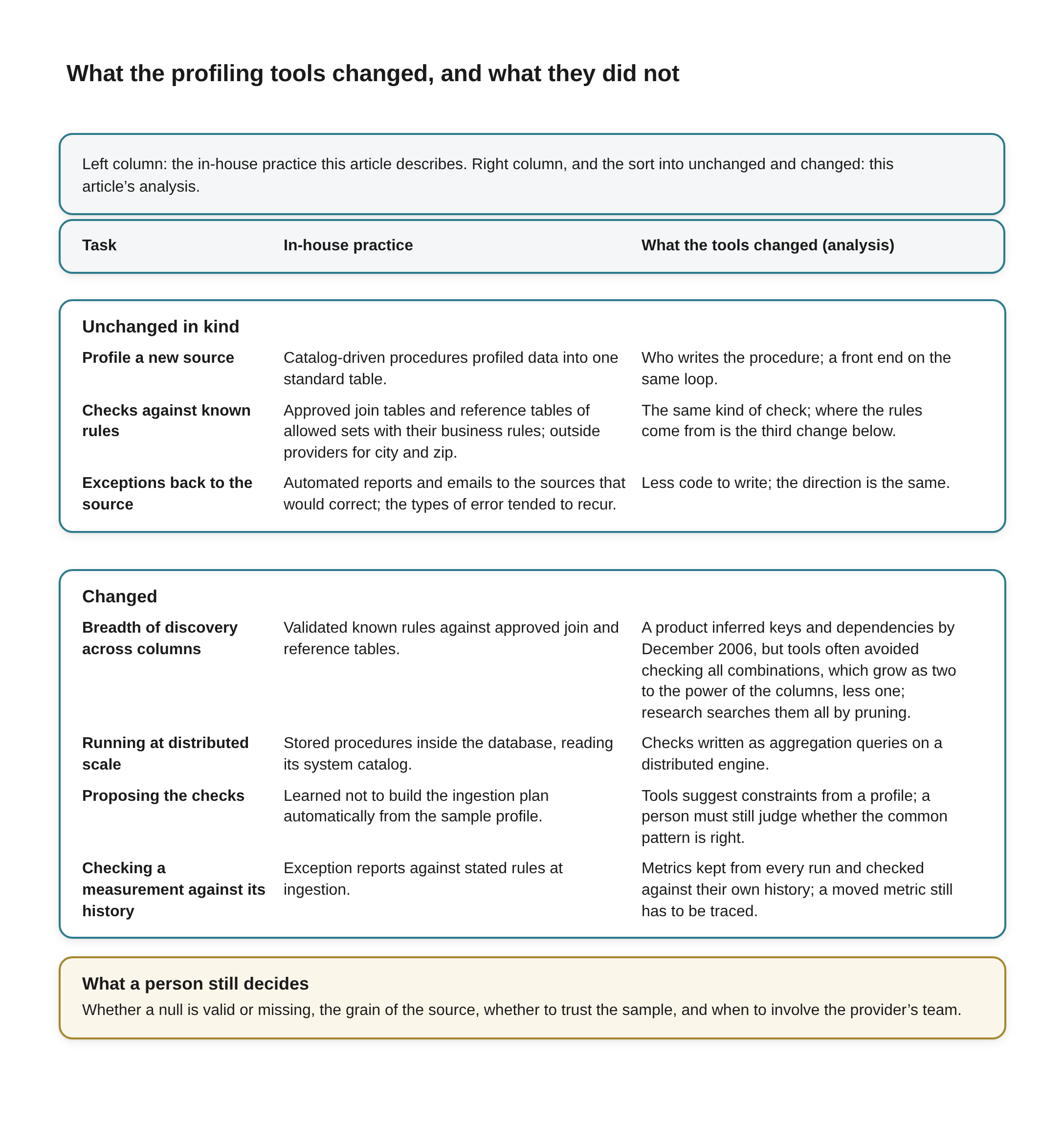
What the profiling tools changed, and what they did not Beneath the title a key reads: Left column: the in-house practice this article describes. Right column, and the sort into unchanged and changed: this article’s analysis.
A table with three column headings, Task, In-house practice and What the tools changed (analysis), in two blocks.
Unchanged in kind
- Profile a new source. In-house practice: Catalog-driven procedures profiled data into one standard table. What the tools changed (analysis): Who writes the procedure; a front end on the same loop.
- Checks against known rules. In-house practice: Approved join tables and reference tables of allowed sets with their business rules; outside providers for city and zip. What the tools changed (analysis): The same kind of check; where the rules come from is the third change below.
- Exceptions back to the source. In-house practice: Automated reports and emails to the sources that would correct; the types of error tended to recur. What the tools changed (analysis): Less code to write; the direction is the same.
Changed
- Breadth of discovery across columns. In-house practice: Validated known rules against approved join and reference tables. What the tools changed (analysis): A product inferred keys and dependencies by December 2006, but tools often avoided checking all combinations, which grow as two to the power of the columns, less one; research searches them all by pruning.
- Running at distributed scale. In-house practice: Stored procedures inside the database, reading its system catalog. What the tools changed (analysis): Checks written as aggregation queries on a distributed engine.
- Proposing the checks. In-house practice: Learned not to build the ingestion plan automatically from the sample profile. What the tools changed (analysis): Tools suggest constraints from a profile; a person must still judge whether the common pattern is right.
- Checking a measurement against its history. In-house practice: Exception reports against stated rules at ingestion. What the tools changed (analysis): Metrics kept from every run and checked against their own history; a moved metric still has to be traced.
A full-width box outlined in amber, headed What a person still decides: Whether a null is valid or missing, the grain of the source, whether to trust the sample, and when to involve the provider’s team.
The first is breadth of discovery across columns. Whether a zip code determines a state is not a question about either column; it is about the pair. The Microsoft task I just cited gives, as an example of what it can report, the strength of the dependency of State on Zip [10], and its request pages describe a wildcard option that, combined with a named column, tests combinations of columns, with a warning that it might result in a large number of computations [10]. A December 2006 IBM white paper describes a product that infers keys and dependency relations from the data and lets the user test permutations of up to nine columns for uniqueness [16]. So by December 2006 at least one commercial product, IBM's, was inferring keys and dependency relations from the data [16]. What I count as the change is breadth: the 2013 overview cited above says the profiling tools of its day often avoided checking all combinations of columns [6], and the research is about searching all of them.
Finding the rules nobody has written down is the harder problem, and a survey of profiling research lists its dependency tasks as unique column combinations, functional dependencies and inclusion dependencies [13]. The trouble is that the candidates multiply. A table with n columns has 2^n minus 1 possible combinations of columns, so thirty columns means more than a billion, and a loop that checks columns one at a time cannot be extended to cover them by writing more of the same query.
The research on the problem is about pruning that space; the same overview calls the results computationally complex to discover [6], and the survey states that discovering all minimal unique column combinations is NP-hard and that dependency discovery is exponential in the worst case [13]. Stated carefully, this exception does not say any product searches every combination: a loop of checks against stated rules never attempts that search, and the research shows it is a search that has to be pruned to be attempted at all. In my own work the answer to whether I needed checks across columns is yes.
Yes, frequently. That's where secondary files and 'approved' join tables existed to validate data was correct. In some of the more complicated cases--such as city and zip matching--we use(d) outsourced data providers like Google to do standardization and validation. For internal validation, we create and maintain reference tables that describe the 'allowed' data sets and the business rules surrounding those restrictions.
These are checks against a known answer: an approved table of allowed combinations, a reference table of allowed sets with the business rules around them, and for the hard cases such as matching a city to a zip code, a provider outside the building. That is validation. The research behind the survey is about something else, which is discovery: finding which dependencies hold in a table when nobody has written them down. I validated what the business had already decided, and I would not claim I went looking for rules nobody had stated. My claim survives for validation and fails for breadth of discovery, and the explosion in candidate column combinations is the reason the failure is real and not a matter of convenience.
The second is scale. The Amazon team that published a data quality system in 2018 describes it as translating the metrics it needs into aggregation queries that run on a distributed engine, so the same declared check can run on a very large data set [14]. The authors say it is designed to scale to billions of rows, provided the constraints are chosen with care [15]. That is not a new idea about what to count. It is a different machine, and in places a different algorithm (sketches, incremental state) [14], doing the counting, and it matters when the data outgrows what a procedure inside one database can cover.
The third is suggestion. The same system profiles a data set and proposes constraints from the profile [14][15]. The procedures were my own, and we maintained the reference tables; a tool that proposes the check moves the first draft of what is worth checking from a person to the data. That is the hazard of the dead end, and the authors name it themselves: they treat suggestion as a human-in-the-loop process, rely on the user to select and validate what it proposes, and warn that a suggested constraint might not hold for future data [14]. A constraint suggested from the data you have will describe the data you have, errors included, and a person still has to decide whether the common pattern is the correct one. The suggestion is still worth having. Reviewing a proposed check is cheaper than writing one from nothing, provided the review is real and not a click.
The fourth is the history of the measurements. The loop as I defined it checks a source against rules someone has stated. The same Amazon system also keeps the quality metrics from successive runs and checks each new value against that history: its authors place no restriction on the detection algorithm, ship simple ones such as a user-defined threshold or a running mean and variance compared with a user-defined bound, and let users plug in their own [14]. That is a check of a measurement against its own past, not against a business rule, and it is a different shape of loop. It flags that a measurement moved. It does not say whether the new value is wrong, or why it moved, and the trace from a moved metric to the process that moved it is the same root cause work as before. What it changes is when you find out. The loop I ran profiled a new source and then caught the records that failed known rules; a watched metric can show a process drifting before any rule fails. Earlier I said that an exception report read as a trend by type is a profile of the source's process. Watching the metrics builds that reading into every run instead of leaving it to whoever thinks to look.
Where the claim stands
The claim I started with, that the only difference is whether the library was written in house or in the public domain, survives for the work I did on single columns, on known rules, and on the exception loop. It does not survive breadth of discovery across many columns, the move from what a procedure inside one database can cover to a distributed engine, tools that propose the checks, or checks of a measurement against its own history. What none of them took is the set of decisions around the profile: whether a null is valid or missing, what the grain is, whether to trust the sample, and when to bring in the people who produce the data. The four exceptions are where I would look first if I were asked what the platform era added. The decisions are where I would look if I were asked what it did not.
References
[1] Microsoft, "Catalog views (Transact-SQL)" and "Mapping system tables to system views (Transact-SQL)," SQL Server documentation. Read 2026-11-15. Cited for the description of catalog views as the most general interface to catalog metadata, and for the mapping of the SQL Server 2000 system tables, including sysobjects and syscolumns, to the system views of SQL Server 2005 and later. https://learn.microsoft.com/en-us/sql/relational-databases/system-catalog-views/catalog-views-transact-sql ; https://learn.microsoft.com/en-us/sql/relational-databases/system-tables/mapping-system-tables-to-system-views-transact-sql
[2] Erhard Rahm and Hong Hai Do, "Data Cleaning: Problems and Current Approaches," IEEE Data Engineering Bulletin 23, no. 4 (2000): 3–13. Read 2026-11-15. Cited for the statement that analysis programs should be used in addition to manual inspection, and for naming Evoke's MigrationArchitect as a commercial profiling tool.
[3] Leo L. Pipino, Yang W. Lee and Richard Y. Wang, "Data Quality Assessment," Communications of the ACM 45, no. 4 (2002): 211–218. doi:10.1145/505248.506010. Read 2026-11-15. Cited for the description of the measures as ad hoc.
[4] Ziawasch Abedjan, Lukasz Golab and Felix Naumann, "Data Profiling: A Tutorial," SIGMOD 2017. doi:10.1145/3035918.3054772. Read in part 2026-11-15 (abstract and introduction). https://hpi.de/oldsite/fileadmin/user_upload/fachgebiete/naumann/publications/PDFs/2017_abedjan_data.pdf
[5] Jack E. Olson, Data Quality: The Accuracy Dimension (Morgan Kaufmann, 2003). Read in part 2026-11-15: only the publisher's description was read, not the book text. Cited for that description.
[6] Felix Naumann, "Data Profiling Revisited," SIGMOD Record 42, no. 4 (2013): 40–49. Read in part 2026-11-15 (introduction and challenges). https://hpi.de/oldsite/fileadmin/user_upload/fachgebiete/naumann/publications/2013/profiling_vision.pdf
[7] "Informatica buys Similarity," The Register (IT-Analysis.com comment), 6 February 2006. Read 2026-11-15. Cited as one analyst's description of Evoke and Axio, not as established market history. https://www.theregister.com/2006/02/06/informatica_similarity_purchase/
[8] Informatica Corporation, Annual Report on Form 10-K for fiscal year 2005. Read 2026-11-15 (the acquisition paragraph). https://capedge.com/filing/1080099/0000891618-06-000094/10K-2005FY
[9] "SWOT: Informatica's Quality Acquisition," Enterprise Systems Journal / TDWI, 1 February 2006. Read 2026-11-15. Cited for Similarity's acquisition of Evoke Software from CSI International in July 2005. https://esj.com/articles/2006/02/01/swot-informaticas-quality-acquisition.aspx
[10] Microsoft, "Data Profiling Task and Viewer," SQL Server Integration Services documentation, and the task's setup and request pages for the key and dependency profiles. Read 2026-11-15. https://learn.microsoft.com/en-us/sql/integration-services/control-flow/data-profiling-task-and-viewer ; https://learn.microsoft.com/en-us/sql/integration-services/control-flow/setup-of-the-data-profiling-task ; https://learn.microsoft.com/en-us/sql/integration-services/control-flow/functional-dependency-profile-request-options-data-profiling-task ; https://learn.microsoft.com/en-us/sql/integration-services/control-flow/candidate-key-profile-request-options-data-profiling-task
[11] dataProfilerR, CRAN package, version 0.2.1 (2026-06-24). Read the package page and reference manual 2026-11-15; the package page lists column type inference first. https://cran.r-project.org/package=dataProfilerR
[12] ydata-profiling documentation. Read 2026-11-15. https://docs.profiling.ydata.ai/latest/
[13] Ziawasch Abedjan, Lukasz Golab and Felix Naumann, "Profiling relational data: a survey," The VLDB Journal 24, no. 4 (2015): 557–581. doi:10.1007/s00778-015-0389-y. Read about three quarters of a mirror copy 2026-11-15 (the task classification and the complexity discussion); the publisher page could not be fetched.
[14] Sebastian Schelter, Dustin Lange, Philipp Schmidt, Meltem Celikel, Felix Biessmann and Andreas Grafberger, "Automating Large-Scale Data Quality Verification," PVLDB 11, no. 12 (2018): 1781–1794. doi:10.14778/3229863.3229867. Read in part 2026-11-15 (abstract, introduction and Sections 3.1 to 3.4). https://www.vldb.org/pvldb/vol11/p1781-schelter.pdf
[15] Sebastian Schelter, Stefan Grafberger, Philipp Schmidt, Tammo Rukat, Mario Kiessling, Andrey Taptunov, Felix Biessmann and Dustin Lange, "Deequ - Data Quality Validation for Machine Learning Pipelines," NeurIPS 2018 workshop paper. Read 2026-11-15. https://cdn.amazon.science/9f/b6/15099d504c54bec20ec6a6c2eb3d/deequ-data-quality-validation-for-machine-learning-pipelines.pdf
[16] IBM Software Group, "Profiling: Take the first step toward assuring data quality," white paper, December 2006. Read 2026-11-15. Describes IBM WebSphere Information Analyzer; cited for key inference, uniqueness tests over permutations of up to nine columns and dependency inference. https://public.dhe.ibm.com/software/data/integration/whitepapers/dataprofiling.pdf